
Ever since I wrote my very visual guide on predicting house prices using automated ml, I’ve been thinking about developing a more realistic use case. I wanted to show how to build a production machine learning system in Azure, with all the tiny and not-so-tiny infrastructure bits that make or break a live project.
Enter Bitcoin. As I’m writing these words the crypto markets have had some wild weeks, with Bitcoin exchange rates going above and beyond 20k USD to break the 40k barrier, before dropping to 34k, then rising again. This is a time when fortunes are made, and lost, as legendary investor Jeremy Grantham likes to say. So, while we’re waiting for the music to stop, let’s at least have some fun shall we? What if we tried predicting which way crypto prices would go? Could we build something accurate enough? 🤨
Well, most likely not. It’s been tried before, and the issue here is that crypto (or stocks, or currency) exchange rates depend on a significant amount of factors, to say the least, and you’d need to identify the factors causing the ups and downs, and you’d need to create features based on them, and make sure they stay relevant over time, etc. Not an easy task.
However, even though I don’t expect the actual forecasting of crypto prices to work in a reliable fashion, it sure sounds like a fun problem to tackle. It’s a good scenario I think for building an end-to-end machine learning system, and it gives me the perfect excuse to go into some of my favorite features of Azure ML. A win-win situation, if you will.

The Plan
As you know, building a production ml system is slightly more complicated than just calling fit and hoping for the best. In today’s article I’ll be showing you how to train a baseline model that’s just useful enough to be dangerous, and then expand on it in a series of future blog posts.
As always, I’ll be using Azure Machine Learning.
Step 1: Data Collection with pandas-datareader
First things first we need to decide what we want to predict. I’d go for something popular but not too popular, if you know what I mean. That rules out Bitcoin, sadly. I wonder what other options are there?
Coinbase to the rescue! Looking at their top cryptocurrencies by market cap, I see Ethereum hanging tight right below Bitcoin. And I remember I’ve heard some good things about Ethereum. Plus, it’s got a cool name. And it’s price has been going up lately, too. This is definitely the cryptocurrency we’re looking for.

Now that we’ve settled on a coin let’s get some historical data to train our model, and the more the better. Luckily, there are several ways to get historic prices for crypto, I find pandas-datareader to be one of the easiest ones to integrate. It supports a variety of data sources too.
If we were to look at, say, Ethereum exchange rates to USD we’d get something like this:
from datetime import datetime
import pandas_datareader as reader

df = reader.get_data_yahoo(['ETH-USD'], start=datetime(2015,7,30))
df
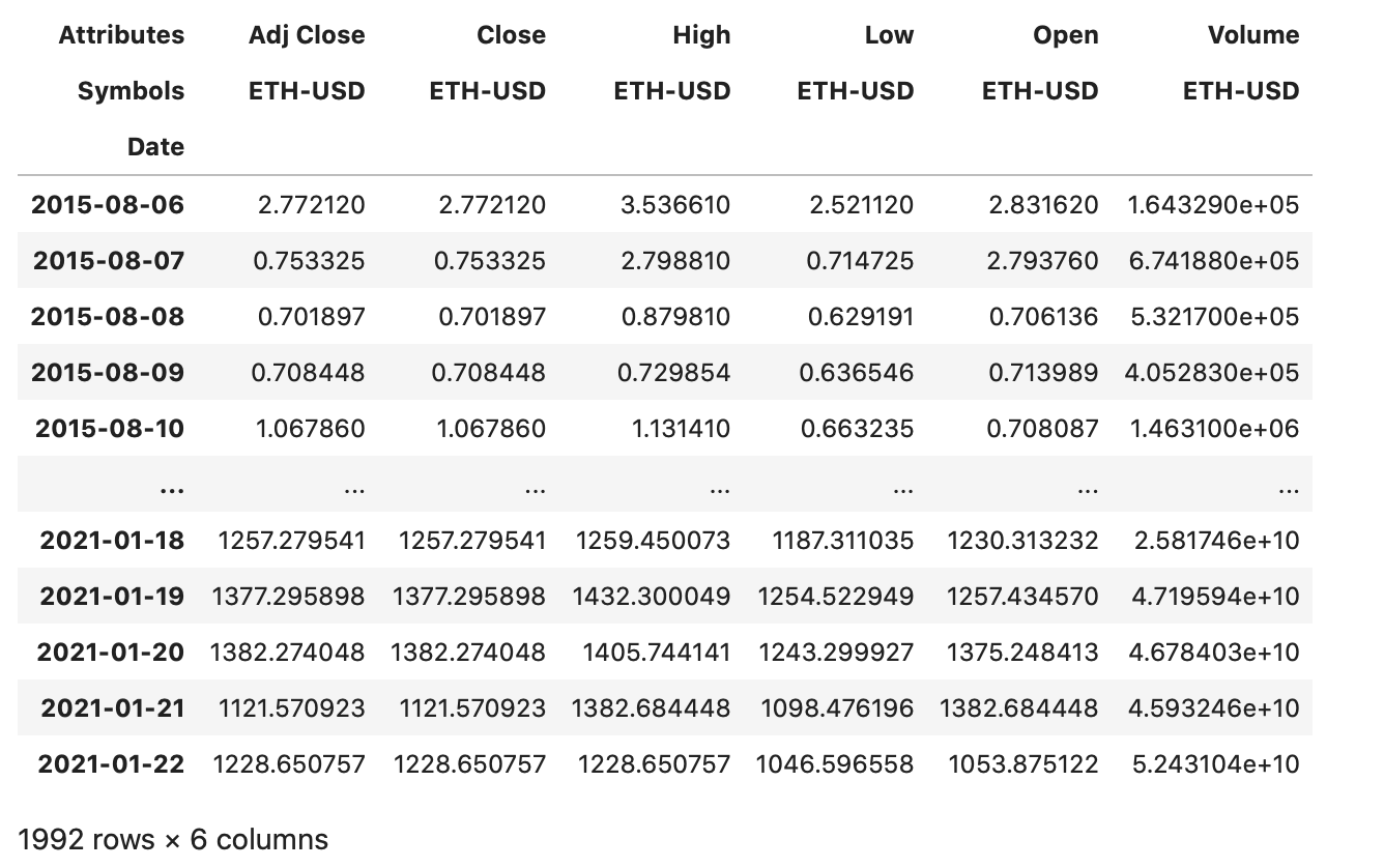
Not bad, we get daily Open/Close/Low/High exchange rates for the past five and a half years, they should be good enough to train a baseline. For now, let’s skip any forecasts of daily highs/lows, and focus on building a model that predicts next day’s closing price.
Step 2: Data Cleaning and Some Light EDA
Now that we’ve gathered a dataset, let’s have a quick look at the data.
import pandas as pd
pd.plotting.register_matplotlib_converters()

print(df.info())

df['Close'].plot(figsize=(16,6))
<class 'pandas.core.frame.DataFrame'>
DatetimeIndex: 1987 entries, 2015-08-06 to 2021-01-22
Data columns (total 6 columns):
(Adj Close, ETH-USD)    1987 non-null float64
(Close, ETH-USD)        1987 non-null float64
(High, ETH-USD)         1987 non-null float64
(Low, ETH-USD)          1987 non-null float64
(Open, ETH-USD)         1987 non-null float64
(Volume, ETH-USD)       1987 non-null float64
dtypes: float64(6)
memory usage: 108.7 KB
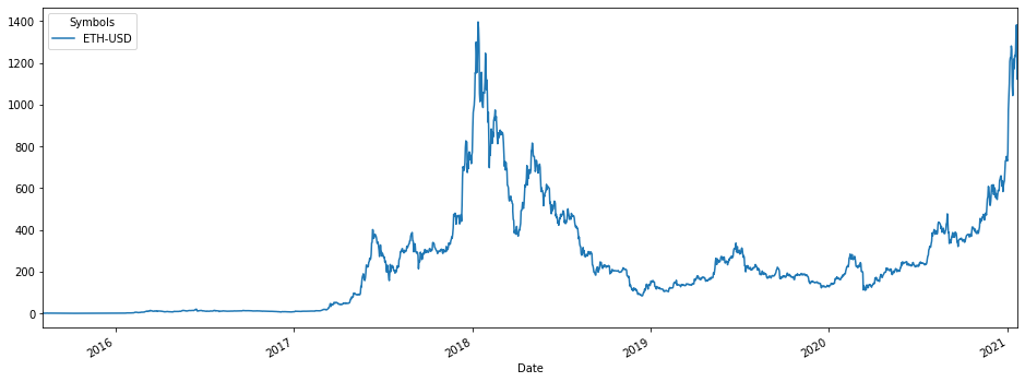
Apart from the very interesting chart above, we can notice a couple of things: there aren’t any null values, but the even though we have 1992 rows in our dataframe, the DateTimeIndex only contains 1987 entries. Houston, we might have a duplicates problem.
We can check if that’s the case using this bit of code from the wiki.
df[df.index.duplicated()]
And of course there are some duplicates which we’ll have to drop, to avoid having any issues down the road.
We’ll also have to drop all other features except the Close rates, otherwise we risk getting a model that learns to predict next day’s Ethereum closing price based on the next day’s highs & lows, and then we’ll have two problems.
df = df[~df.index.duplicated(keep='first')]
df = df['Close']
Step 3: Training a Forecasting Model with Azure Automated ML
The fastest way to train a baseline model would be using some flavor of automated ml, and we have just the thing:
Automated machine learning, also referred to as automated ML or AutoML, is the process of automating the time consuming, iterative tasks of machine learning model development. It allows data scientists, analysts, and developers to build ML models with high scale, efficiency, and productivity all while sustaining model quality. Automated ML in Azure Machine Learning is based on a breakthrough from our Microsoft Research division.
Traditional machine learning model development is resource-intensive, requiring significant domain knowledge and time to produce and compare dozens of models. With automated machine learning, you’ll accelerate the time it takes to get production-ready ML models with great ease and efficiency.
Basically, even though you probably won’t get the best model you can get by using automated ml, you’ll get one that’s good enough, and you’ll get it with little enough effort, Pareto principle and all that.
Prerequisites
As I was saying, last time I showed how to use Automated ML directly from Azure ML studio, so today I’ll show you an more flexible way, using the SDK. Just make sure to install it as per the official instructions and don’t forget to include the automl optional package. Or, you can just create a new Azure Notebook and follow along, it’ll have (almost) all the packages you need.
First, we’ll need to register our dataframe in ML Studio’s Dataset store, where it can be accessed easily from compute instances running in the cloud. Said compute instances which we’ll also have to create.
To see just how good our model’s forecasts actually are, I’ll drop the last two days of data just before registering the dataset. This means our model won’t have access to them while training, and we’ll be able to compare their true exchange rates with the ones our model predicts.
You might also notice that I’m resetting the dataframe’s index, and this is because Automated ML cannot handle DateTime indexes just yet, requiring datasets used for forecasting to have a datetime column instead of a datetime index.
from azureml.core import Workspace, Dataset

ws = Workspace.from_config()
datastore = ws.get_default_datastore()

df_sans_last_two_days = df[:-2]
df_sans_last_two_days.reset_index(inplace=True)
training_data = Dataset.Tabular.register_pandas_dataframe(
    df_sans_last_two_days, datastore, 'EthereumRates')
Pay special attention to the Workspace.from_config() line. This may or may not work depending on whether you’re running in an Azure notebook or not. If not, you’ll need to download the configuration directly from the Azure portal, see this article for more details.
When creating the compute target, it’s best to check if it already exists and if it does, use that instance instead to avoid any issues.
from azureml.core.compute import ComputeTarget, AmlCompute

compute_name = 'Spock'

if compute_name in ws.compute_targets:
    compute_target = ws.compute_targets[compute_name]
    if compute_target and type(compute_target) is AmlCompute:
        print(f'Using existing compute: {compute_name}')
else:
    print(f'Creating new compute: {compute_name}')
    provisioning_config = AmlCompute.provisioning_configuration(
        vm_size = 'Standard_F4s_v2',
        min_nodes = 0,
        max_nodes = 4)

    compute_target = ComputeTarget.create(ws, compute_name, provisioning_config)

    compute_target.wait_for_completion(show_output=True)
Configuration
Now, and this is the fun part - we’ll configure Automated ML to the best of our knowledge, and see how the different configuration options affect the performance of the resulting model.
Looking at the code below, some of the settings are self explanatory while others might need some additional details. I’ve summarized some of the most important ones below, and you can find out more about them in the docs available here and here.
from azureml.train.automl import AutoMLConfig
from azureml.automl.core.forecasting_parameters import ForecastingParameters

forecasting_parameters = ForecastingParameters(
    time_column_name='Date',
    freq='1D',
    forecast_horizon=1,
    feature_lags='auto',
    target_lags=[7],
    use_stl=None,
    country_or_region_for_holidays='US',
)
- freq - the dataset’s frequency, which in our case is
daily - forecast_horizon - how many periods forward to forecast, setting this to
1since we only want to forecast day-ahead prices - target_lags - how many past periods to use as features, useful especially when the data is autocorrelated (and in our case it is, trust me on that) - I’ll set this to lag
one weekfor now, keep in mind that we can configure it to lag multiple columns - use_stl - extract seasonality and trend from the time series and use them as features; from a quick look at the chart above, I can’t say I see a big seasonality component so let’s set it to
None - country_or_region_for_holidays - if set, Automated ML’s featurizer will create features for each and every holiday in the specified country and/or region; I expect holidays to influence the crypto prices to some extent, so I’ll set it to
US
automl_config = AutoMLConfig(
    task = "forecasting",
    primary_metric='normalized_root_mean_squared_error',

    training_data = training_data,
    label_column_name = 'ETH-USD',
    n_cross_validations=7,

    enable_early_stopping=True,
    early_stopping_n_iters=20,
    max_concurrent_iterations=4,
    iteration_timeout_minutes=5,

    compute_target=compute_target,
    forecasting_parameters=forecasting_parameters
)
- task and normalized_root_mean_squared_error - apart from the classic regression & classification tasks, Azure Automated ML has dedicated support for forecasting tasks, so we’ll tell it to use it. We’ll also configure it to use
normalized RMSEwhile evaluating models - after all, our goal is to minimize price errors - enable_early_stopping and early_stopping_n_iters - these are two very cool features, basically configuring our experiment to run until our RMSE doesn’t improve over
20 iterations, at which point consider the job done and finish up - max_concurrent_iterations - use up to
4nodes from our trusty compute instance, this setting directly affects the speed with which we get results - n_cross_validations - you’ll have to pay special attention to this setting since this ain’t your regular k-fold cross validation, no sirree. When forecasting, Automated ML uses Rolling Origin Cross Validation, dividing the series into training and validation data by using an origin time point and sliding it for each fold. This is great, because classic cross validation is not ideal for time series, but at the same time not so great, because it only evaluates the model on
7days.
Bombs away 💣.
from azureml.core import Experiment

experiment = Experiment(ws, "AutoML-Forecasting")
run = experiment.submit(automl_config, show_output=True)

best_run, best_model = run.get_output()
Now that you’ve run the code, better start brewing some coffee ‘cause this might take a while. In my tests it takes somewhere between 20 to 30 minutes to run, but as with all fine things in life, ymmv.

Roughly after drinking that third espresso you’ll (hopefully) notice the experiment has finally ended, printing something similar to the output below.
ITERATION   PIPELINE                               DURATION      METRIC      BEST
0   RobustScaler LassoLars                         0:00:50       0.1201    0.1201
1   RobustScaler DecisionTree                      0:00:54       0.0953    0.0953
2   StandardScalerWrapper DecisionTree             0:00:57       0.1171    0.0953
3   RobustScaler DecisionTree                      0:00:54       0.1012    0.0953
4   StandardScalerWrapper ElasticNet               0:00:50       0.1160    0.0953
5   MinMaxScaler DecisionTree                      0:00:51       0.1662    0.0953
6   MinMaxScaler ElasticNet                        0:00:54       0.1117    0.0953
7   StandardScalerWrapper DecisionTree             0:00:53       0.1663    0.0953
8   StandardScalerWrapper DecisionTree             0:00:56       0.1043    0.0953
9   RobustScaler DecisionTree                      0:00:50       0.0981    0.0953
10   RobustScaler ElasticNet                        0:00:57       0.1157    0.0953
11   RobustScaler DecisionTree                      0:00:50       0.0948    0.0948
12   RobustScaler DecisionTree                      0:00:50       0.1663    0.0948
13   StandardScalerWrapper DecisionTree             0:00:53       0.0969    0.0948
14   MinMaxScaler DecisionTree                      0:00:54       0.0948    0.0948
15   MinMaxScaler DecisionTree                      0:00:53       0.0902    0.0902
16   RobustScaler DecisionTree                      0:00:54       0.0948    0.0902
17   StandardScalerWrapper DecisionTree             0:00:53       0.1171    0.0902
18   MinMaxScaler DecisionTree                      0:00:48       0.0948    0.0902
19   StandardScalerWrapper LassoLars                0:00:54       0.1203    0.0902
20   MinMaxScaler DecisionTree                      0:00:53       0.0948    0.0902
21   StandardScalerWrapper DecisionTree             0:00:47       0.1012    0.0902
22   StandardScalerWrapper RandomForest             0:01:09       0.2653    0.0902
23   MaxAbsScaler RandomForest                      0:01:03       0.1106    0.0902
24   MinMaxScaler GradientBoosting                  0:01:06       0.2029    0.0902
25   StandardScalerWrapper DecisionTree             0:00:54       0.1924    0.0902
26   MinMaxScaler DecisionTree                      0:01:02       0.1663    0.0902
27   MinMaxScaler ExtremeRandomTrees                0:00:54       0.2532    0.0902
28   MinMaxScaler RandomForest                      0:01:06       0.1490    0.0902
30   StandardScalerWrapper DecisionTree             0:00:50       0.4549    0.0902
31   MaxAbsScaler GradientBoosting                  0:00:47       0.3129    0.0902
29   MaxAbsScaler RandomForest                      0:01:40       0.2314    0.0902
32   MinMaxScaler RandomForest                      0:01:03       0.1696    0.0902
33   MaxAbsScaler RandomForest                      0:00:59       0.1082    0.0902
34   MaxAbsScaler ExtremeRandomTrees                0:00:53       0.1122    0.0902
35   SparseNormalizer DecisionTree                  0:00:54       0.1007    0.0902
36   MinMaxScaler GradientBoosting                  0:00:59       0.1696    0.0902
37   RobustScaler RandomForest                      0:00:53       0.3166    0.0902
38   RobustScaler GradientBoosting                  0:00:50       0.6045    0.0902
40   RobustScaler DecisionTree                      0:00:50       0.0989    0.0902
41   StandardScalerWrapper ExtremeRandomTrees       0:01:09       0.0936    0.0902
42   MaxAbsScaler RandomForest                      0:01:06       0.2426    0.0902
43   MinMaxScaler GradientBoosting                  0:00:50       0.0912    0.0902
44                                                  0:00:16          nan    0.0902
45                                                  0:00:15          nan    0.0902
46    VotingEnsemble                                0:01:46       0.0818    0.0818
Let’s take the best model - that pretty little VotingEnsemble - for a spin and see how it handles.
P.S. if you want to try the next part without having to run Automated ML EVERY.SINGLE.TIME, use this snippet to load the latest model available.
from azureml.core import Experiment
from azureml.train.automl.run import AutoMLRun

experiment = Experiment(ws, "AutoML-Forecasting")
runs = list(experiment.get_runs())

run = AutoMLRun(experiment, runs[0].id)
best_run, best_model = run.get_output()
Predicting the Future
Now, before we use the model for anything, we need to prepare a dataframe with a single Date column containing the dates we want to make forecasts for. That’s just how it works. There are a couple of things you need to keep in mind here:
- The first day for which we want forecasts has to be immediately following the last day of the training data. This means that if you’ve trained your model on data up to and including
2021-01-21like I did, then you’ll need to have2021-01-22as the first forecast target. - You can actually forecast more than 1 day, by using the model’s
forecastmethod. Callingforecastwill apply the forecasting model for each and every date, starting at the forecast origin and then successively forecasting each day up until the last one. It’s quite cool.
from datetime import datetime

range = pd.date_range(datetime(2021,1,22), datetime(2021,1,30))

forecast_df = pd.DataFrame({ 'Date': range })
Now that we’ve built the dataset, using the model is quite straightforward - we’ll just call forecast and this time, we can hope for the best 🤞.
forecast, transformed_df = best_model.forecast(forecast_df)
We get two things out of forecast, first one being an array with the forecasted values, and the second one being the transformed input dataframe, just in case you wanted to see exactly how it was processed by the featurizer.
Let’s look at the forecast first, and then compare it with the exchange rates from our two held out days.
Jan 25 Edit: I’ve updated the chart with the latest actuals so you can see how the difference gets amplified over time
pretty_df = forecast_df.copy().set_index('Date')
pretty_df['ETH-USD-forecast'] = forecast
pretty_df['ETH-USD'] = df['ETH-USD']

pretty_df[['ETH-USD', 'ETH-USD-forecast']].plot(figsize=(16,6))
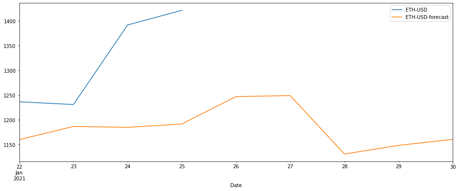
Ouch. 🤕
The coming days should speak more about how well it performs, but so far it certainly looks like there’s room for improvement. That’s good news, it means I’ll have something to explore in the next posts of this series, so yay for me I guess?
Until then, you should definitely try this out yourself. Copy the code, tweak the settings (have you tried multiple lags? or generating holiday features for CN?), let it run for a longer time. See what happens. But whatever you do, just don’t use it as guidance for buying crypto, that would just break my little heart.
Epilogue: Analyzing Model Performance
Looking at the actuals versus forecasted chart, it does look like our model doesn’t work that well. But what if it’s just a fluke? What if it’s a particularly vicious streak of bad luck?
Luckily, Automated ML computes a series of performance metrics for each and every model it trains, and we can access those metrics easily, using the RunDetails widget.
from azureml.widgets import RunDetails

RunDetails(best_run).show()
First thing we’ll look at is the actual Mean Absolute Error in the Metrics tab, this should tell us just how bad our model messes up, on average.
mean_absolute_error 114.18599192085286
With a mean error of ~114.16, our “performance” is definitely more than just a fluke - it means our model will, on average, be 114 USD off when forecasting exchange rates.
The charts below repeat that sentiment, with the Predicted vs. True graph showing a “less than optimal” relationship between the actual and predicted values, and the Residuals graph pointing toward our model’s tendency to consistently predict values lower than the actual values (go here for a more in-depth explanation of those metrics).
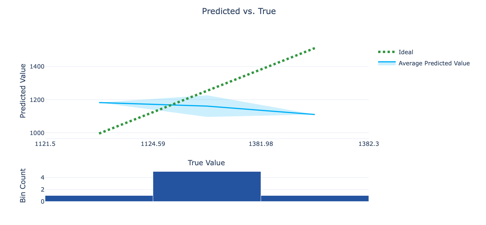
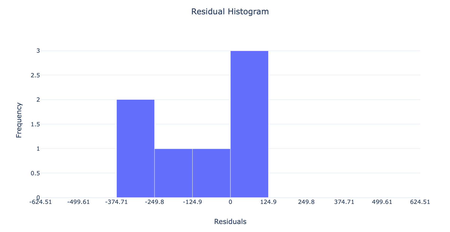
All in all, we’ve got work to do. But don’t worry, it’ll be fun.
Coming Your Way in 2021
Hope you’ve enjoyed the first in this series of articles, I plan to gradually expand and develop this concept into a full fledged app and document each step of the process along the way.
Here are some of the improvements I have planned for the coming months:
- Scheduling Automated ML to run daily using Azure ML pipelines
- Removing the dependency on Automated ML for retraining
- Continually monitoring the live model’s forecasts
- Integration with other APIs and adding more features
- Hyperparameter optimization with HyperDrive
If you’ve enjoyed this article, I’d appreciate it if you shared the Twitter thread:
I've started writing a series of articles about building production machine learning systems in #Azure, using crypto price prediction as thinly veiled excuse to do it. 🧵https://t.co/xySDPbbq1s
— Vlad Iliescu (@vladiliescu) January 25, 2021
Or if you’re feeling particularly adventurous, join my email list and you’ll be the first to know whenever I publish something new. See you! 👋